I had a dream one night where a blackbird was talking in human language. When I woke up there was actually a blackbird singing outside the window. Its inflections were curiously speech-like. The dreaming mind only needed to imagine a bunch of additional harmonics to form phonemes and words. One was left wondering if speech could be transformed into a blackbird song by isolating one of the harmonics...
One way to do this would be to:
Find the instantaneous fundamental frequency and amplitude of the speech. For example, filter the harmonics out and use an FM demodulator to find the frequency. Then find the signal envelope amplitude by AM demodulation.
Generate a new wave with similar amplitude variations but greatly multiplied in frequency.
A proof-of-concept script using the Perl-SoX-csdr command-line toolchain is available (source code here). The result sounds surprisingly blackbird-like. Even the little trills are there, probably as a result of FM noise or maybe vocal fry at the end of sentences. I got the best results by speaking slowly and using exaggerated inflection.
Someone hinted that the type of intonation used in certain automatic announcements is perfect for this kind of conversion. And it seems to be true! Here, a noise gate and reverb has been added to the result to improve it a little:
And finally, a piece of sound art where this synthetic blackbird song is mixed with a subtle chord and a forest ambience:
Think of the possibilities: A simultaneous interpreter for talking to birds. A tool for dubbing talking birds in animation or live theatre. Entertainment for cats.
What other birds could be done with a voice changer like this? What about croaky birds like a duck or a crow?
I play 1980s games, mostly Super Mario Bros., on the Nintendo NES console. It would be great to be able to capture live video from the console for recording speedrun attempts. Now, how to make the 1985 NES and the 2013 MacBook play together, preferably using hardware that I already have? This project diary documents my search for the answer.
Here's a spoiler – it did work:
Things that I tried first
A capture device
Video capture devices, or capture cards, are devices specially made for this purpose. There was only one cheap (~30€) capture device for composite video available locally, and I bought it, hopingly. But it wasn't readily recognized as a video device on the Mac, and there seemed to be no Mac drivers available. Having already almost capped my budget for this project I then ordered a 5€ EasyCap device from eBay, as there was some evidence of Mac drivers online. The EasyCap was still making its way to Finland as of this writing, so I continued to pursure other routes.
PS: When the device finally arrived, it sadly seemed that the EasyCapViewer-Fushicai software only supports opening this device in NTSC mode. There's PAL support in later commits in the GitHub repo, but the project is old and can't be compiled anymore as Apple has deprecated QuickTime.
Even when they do work, a downside to many cheap capture devices is that they can only capture at half the true framerate (that is, at 25 or 30 fps).
CRT TV + DSLR camera
The cathode-ray tube television that I use for gaming could be filmed with a digital camera. This posed interesting problems: The camera must be timed appropriately so that a full scan is captured in every frame, to prevent temporal aliasing (stripes). This is why I used a DSLR camera with a full manual mode (Canon EOS 550D in this case).
For the 50 Hz PAL television screen I used a camera frame rate of 25 fps and an exposure time of 1/50 seconds (set by camera limitations). The camera will miss every other frame of the original 50 fps video, but on the other hand, will get an evenly lit screen every time.
A Moiré pattern will also appear if the camera is focused on the CRT shadow mask. This is due to intererence between two regular 2D arrays, the shadow mask in the TV and the CCD array in the camera. I got rid of this by setting the camera on manual focus and defocusing the lense just a bit.
This produced surprisingly good quality video, save for the slight jerkiness caused by the low frame rate (video). This setup was good for one-off videos; However, I could not use this setup for live streaming, because the camera could only record on the SD card and not connect to the computer directly.
LCD TV + webcam
An old LCD TV that I have has significantly less flicker than the CRT, and I could have live video via the webcam. But the Microsoft LifeCam HD-3000 that I have had only a binary option for manual exposure (pretty much "none" and "lots"). Using the higher setting the video was quite washed out, with lots of motion blur. The lower setting was so fast that it looked like the LCD had visible vertical scanning. Brightness was also heavily dependent on viewing angle, which caused gradients over the image. I had to film at a slightly elevated angle so that the upper part of the image wouldn't go too dark, and this made the video look like a bootleg movie copy.
Composite video
Now to capturing the actual video signal. The NES has two analog video outputs: one is composite video and the other an RF modulator, which has the same composite video signal modulated onto an AM carrier in the VHF television band plus a separate FM audio carrier. This is meant for televisions with no composite video input: the TV sees the NES as an analog TV station and can tune to it.
In composite video, information about brightness, colour, and synchronisation is encoded in the signal's instantaneous voltage. The bandwidth of this signal is at least 5 MHz, or 10 MHz when RF modulated, which would require a 10 MHz IQ sampling rate.
I happen to have an Airspy R2 SDR receiver that can listen to VHF and take 10 million samples per second - could it be possible? I made a cable that can take the signal from the NES RCA connector to the Airspy SMA connector. And sure enough, when the NES RF channel selector is at position "3", a strong signal indeed appears on VHF television channel 3, at around 55 MHz.
Software choices
There's already an analog TV demodulator for SDRs - it's a plugin for SDR# called TVSharp. But SDR# is a Windows program and TVSharp doesn't seem to support colour. And it seemed like an interesting challenge to write a real-time PAL demodulator myself anyway.
I had been playing with analog video demodulation recently because of my HDMI Tempest project (video). So I had already written a C++ program that interprets a 10 Msps digitised signal as greyscale values and sync pulses and show it live on the screen. Perhaps this could be used as a basis to build on. (It was not published, but apparently there is a similar project written in Java, called TempestSDR)
Data transfer from the SDR is done using airspy_rx from airspy-tools. This is piped to my program that reads the data into a buffer, 256 ksamples at a time.
Automatic gain control is an important part of demodulating an AM signal. I used liquid-dsp's AGC by feeding it the maximum amplitude over every scanline period; this roughly corresponds to sync level. This is suboptimal, but it works in our high-SNR case. AM demodulation was done using std::abs() on the complex-valued samples. The resulting real value had to be flipped from 1, because TV is transmitted "inverse AM" to save on the power bill. I then scaled the signal so that black level was close to 0, white level close to 1, and sync level below 0.
I use SDL2 to display the video and OpenCV for pixel addressing, scaling, cropping, and YUV-RGB conversions. OpenCV is an overkill dependency inherited from the Tempest project and SDL2 could probably do all of those things by itself. This remains TODO.
Removing the audio
The captured AM carrier seems otherwise clean, but there's an interfering peak on the lower sideband side at about –4.5 MHz. I originally saw it in the demodulated signal and thought it would be related to colour, as it's very close to the PAL chroma subcarrier frequency of 4.43361875 MHz. But when it started changing frequency in triangle-wave shapes, I realized it's the audio FM carrier. Indeed, when it is FM demodulated, beautiful NES music can be heard.
The audio carrier is actually outside this 10 MHz sampled bandwidth. But it's so close to the edge (and so powerful) that the Airspy's anti-alias filter cannot sufficiently attenuate it, and it becomes folded, i.e. aliased, onto our signal. This caused visible banding in the greyscale image, and some synchronization problems.
I removed the audio using a narrow FIR notch filter from the liquid-dsp library. Now, the picture quality is very much acceptable. Minor artifacts are visible in narrow vertical lines because of a pixel rounding choice I made, but they can be ignored.
Decoding colour
PAL colour is a bit complicated. It was designed in the 1960s to be backwards compatible with black-and-white TV receivers. It uses the YUV colourspace, the Y or "luminance" channel being a black-and-white sum signal that already looks good by itself. Even if the whole composite signal is interpreted as Y, the artifacts caused by colour information are bearable. Y also has a lot more bandwidth, and hence resolution, than the U and V (chrominance) channels.
U and V are encoded in a chrominance subcarrier in a way that I still haven't quite grasped. The carrier is suppressed, but a burst of carrier is transmitted just before every scanline for reference (so-called colour burst).
Turns out that much of the chroma information can be recovered by band-pass filtering the chrominance signal, mixing it down to baseband using a PLL locked to the colour burst, rotating it by a magic number (chroma *= std::polar(1.f, deg2rad(170.f))), and plotting the real and imaginary parts of this complex number as the U and V colour channels. This is similar to how NTSC colour is demodulated.
In PAL, every other scanline has its chrominance phase shifted (hence the name, Phase Alternating [by] Line). I couldn't get consistent results demodulating this, so I skipped the chrominance part of every other line and copied it from the line above. This doesn't even look too bad for my purposes. However, there seems to be a pre-echo in UV that's especially visible on a blue background (most of SMB1 sadly), and a faint stripe pattern on the Y channel, most probably crosstalk from the chroma subcarrier that I left intact for now.
I used liquid_firfilt to band-pass the chroma signal, and liquid_nco to lock onto the colour burst and shift the chroma to baseband.
Let's play Tetris!
Latency
It's not my goal to use this system as a gaming display; I'm still planning to use the CRT. However, total buffer delays are quite small due to the 10 Msps sampling rate, so the latency from controller to screen is pretty good. The laptop can also easily decode and render at 50 fps, which is the native frame rate of the PAL NES. Tetris is playable up to level 12!
Using a slow-mo phone camera, I measured the time it takes for a button press to make Mario jump. The latency is similar to that of a NES emulator:
Method
Frames @240fps
Latency
RetroArch emulator
28
117 ms
PAL NES + Airspy SDR
26
108 ms
PAL NES + LCD TV
20
83 ms
Maybe you now notice that the CRT is not listed here. That's because before I could make these measurements a funny sound was heard from inside the TV and a picture has never appeared since.
Performance considerations
A 2013 MacBook Pro is perhaps not the best choice for dealing with live video to begin with. But I want to be able to run the PAL decoder and a screencap / compositing / streaming client on the same laptop, so performance is even more crucial.
When colour is enabled, CPU usage on this quad-core laptop is 110% for palview and 32% for airspy_rx. The CPU temperature is somewhere around 85 °C. Black-and-white decoding lowers palview usage to 84% and CPU temps to 80 °C. I don't think there's enough cycles left for a streaming client just yet. Some CPU headroom would be nice as well; a resync after dropped samples looks quite nasty, and I wouldn't want that to happen very often.
Profiling reveals that the most CPU-intensive tasks are those related to FIR filtering. FIR filters are based on convolution, which is of high computational complexity, unless done in hardware. FFT convolution can also be faster, but only when the kernel is relatively long.
I've thought of having another computer do the Airspy transfer, audio notch filtering, and AM demodulation, and then transmit this preprocessed signal to the laptop via Ethernet. But my other computers (Raspberry Pi 3B+ and a Core 2 Duo T7500 laptop) are not nearly as powerful as the MacBook.
Instead of a FIR bandpass filter, a so-called chrominance comb filter is often used to separate chrominance from luminance. This could be realized very efficiently as a linear-complexity delay line. This is a promising possibility, but so far my experiments have had mixed results.
There's no source code release for now (Why? FAQ), but if you want some real-time coverage of this project, I did a multi-threaded tweetstorm:
one,
two,
three.
Lately my listening activities have focused on two-way FM radio. I'm interested in automatic monitoring and visualization of multiple channels simultaneously, and classifying transmitters. There's a lot of in-band signaling to be decoded! This post shall demonstrate this diversity and also explain how my listening station works.
Background: walkie-talkies are fun
The frequency band I've recently been listening to the most is called PMR446. It's a European band of radio frequencies for short-distance UHF walkie-talkies. Unlike ham radio, it doesn't require licenses or technical competence – anyone with 50€ to spare can get a pair of walkie-talkies at the department store. It's very similar to FRS in the US. It's quite popular where I live.
The short-distance nature of PMR446 is what I find perhaps most fascinating: in normal conditions, everything you hear has been transmitted from a 2-kilometer (1.3-mile) radius. Transmitter power is limited to 500 mW and directional antennas are not allowed on the transmitter side. But I have a receive-only system and a my only directional antenna is for 450 MHz, which is how I originally found these channels.
Roger beep
The roger beep is a short melody sent by many hand-held radios to indicate the end of transmission.
The end of transmission must be indicated, because two-way radio is 'half-duplex', which means only one person can transmit at a time. Some voice protocols solve the same problem by mandating the use of a specific word like 'over'; others rely on the short burst of static (squelch tail) that can be heard right after the carrier is lost. Roger beeps are especially common in consumer radios, but I've heard them in ham QSOs as well, especially if repeaters are involved.
Other signaling on PMR
PMR also differs from ham radio in that many of its users don't want to hear random people talking on the same frequency; indeed, many devices employ tones or digital codes designed to silence unwanted conversations, called CTCSS, DCS, or coded squelch. They are very low-frequency tones that can't usually be heard at all because of filtering. These won't prevent others from listening to you though; anyone can just disable coded squelch on their device and hear everyone else on the channel.
Many devices also use a tone-based system for preventing the short burst of static, that classic walkie-talkie sound, from sounding whenever a transmission ends. Baofeng calls these squelch tail elimination tones, or STE for short. The practice is not standardized and I've seen several different sub-audible frequencies being used in the wild, namely 55, 62, and 260 Hz. (Edit: As correctly pointed out by several people, another way to do this is to reverse the phase of the CTCSS tone in the end, called a 'reverse burst'. Not all radios use it though; many opt to send a 55 Hz tone instead, even when they are using CTCSS.)
Some radios have a button called 'alarm' that sends a long, repeating melody resembling a 90s mobile phone ring tone. These melodies also vary from one radio to the other.
My receiver
I have a system in place to alert me whenever there's a strong enough signal matching an interesting set of parameters on any of the eight PMR channels. It's based on a Raspberry Pi 3B+ and an Airspy R2 SDR receiver. The program can play the live audio of all channels simultaneously, or one could be selected for listening. It also has an annotated waterfall view that shows traffic on the band during the last couple of hours:
The computer is a headless Raspberry Pi with only SSH connectivity; that's why it's in text mode. Also, text-mode waterfall plots are cool!
The coloured bars indicate signal strength (colour) and the duty factor (pattern). The numbers around the bars are decoded squelch codes, STEs and roger beeps. Uncertain detections are greyed out. In this view we've detected roger beeps of type 'a1' and 'a2'; a somewhat rare 62 Hz STE tone; and a ring tone, or alarm (RNG).
Because squelch codes are designed to be read by electronic circuits and their frequencies and codewords are specified exactly, writing a digital decoder for them was somewhat straightforward. Roger beeps and ring tones, on the other hand, are only meant for the human listener and detecting them amongst the noise took a bit more trial-and-error.
Melody detection algorithm
The melody detection algorithm in my receiver is based on a fast Fourier transform (FFT). When loss of carrier is detected, the last moments of the audio are searched for tones thusly:
The audio buffer is divided up into overlapping 60-millisecond Hann-windowed slices.
Every slice is Fourier transformed and all peak frequencies (local maxima) are found. Their center frequencies are refined using Gaussian peak interpolation (Gasior & Gonzalez 2004). We need this, because we're only going to allow ±15 Hz of frequency error.
The time series formed by the strongest maxima is compared to a list of pre-defined 'tone signatures'. Each candidate tone signature gets a score based on how many FFT slices match (+) corresponding slices of the tone signature. Slices with too much frequency error subtract from the score (–).
Most tone signatures have one or more 'quiet zones', the quietness of which further contributes to the score. This is usually placed after the tone, but some tones may also have a pause in the middle.
The algorithm allows second and third harmonics (with half the score), because some transmitters may distort the tones enough for these to momentarily overpower the fundamental frequency.
Every possible time shift (starting position) inside the 1.5-second audio buffer is searched.
The tone signature with the best score is returned, if this score exceeds a set threshold.
This algorithm works quite well. It's not always able to detect the tones, especially if part of the melody is completely lost in noise, but it's good enough to be used for waterfall annotation. False positives are rare; most of them are detections of very short tone signatures that only consist of one or two beeps. My test dataset of 92 recorded transmissions yields only 5 false negatives and no false positives.
For example, this noisy recording:
was succesfully recognized as having a ringtone (RNG), a roger beep of type a1, and CTCSS code XA:
Naming and classification
Because I love classifying stuff I've had to come up with a system for naming these roger tones as well. My current system uses a lower-case letter for classifying the tone into a category, followed by a number that differentiates similar but slightly different tones. This is a work in progress, because every now and then a new kind of tone appears.
My goal would be to map the melodies to specific manufacturers. I've only managed to map a few. Can you recognise any of these devices?
Class
Identified model
Recording
a
Cobra AM845 (a1)
c
Motorola TLKR T40 (c1)
d
?
e
?
h
Baofeng UV-5RC
i
?
I didn't list them all here, but there are even more samples. I've added some alarm tones there as well, and a list of all the tone signatures that I currently know of. (Why no full source code? FAQ)
In my rx log I also have an emoji classification system for CTCSS codes. This way I can recognize a familiar transmission faster. A few examples below (there are 38 different CTCSS codes in total):
Future directions
There are mainly just minor bugs in my project trello at the moment, like adding the aforementioned emoji. But as the RasPi is not very powerful the DSP chain could be made more efficient. Sometimes a block of samples gets dropped. Currently it uses a bandpass-sampled filterbank to separate the channels, exploiting aliasing to avoid CPU-intensive frequency shifting altogether:
This is quite fast. But the 1:20 decimation from the Airspy IQ data is done with SoX's 1024-point FIR filter and could possibly be done with fewer coefficients. Also, the RasPi has four cores, so half of the channels could be demodulated in a second thread. Currently all concurrency is thanks to SoX and pmrsquash being different processes.
OpenCV is a pretty versatile C++ computer vision library. Because I use it every day it has also become my go-to tool for creating simple animations at pixel level, for fun, and saving them as video files. This is not one of its core functions but happens to be possible using its GUI drawing tools.
Below we'll take a look at some video art I wrote for a music project. It goes a bit further than just line drawings but the rest is pretty much just flavouring. As you'll see, creating images in OpenCV has a lot in common with how you would work with layers and filters in an image editor like GIMP or Photoshop.
Setting it up
It doesn't take a lot of boilerplate to initialize an OpenCV project. Here's my minimal CMakeLists.txt:
This will also initialize everything to zero, i.e. black.
Now we can draw our graphics!
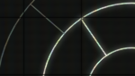
I had an initial idea of an endless cascade of concentric rings each rotating at a different speed. There might be color and brightness variations as well but otherwise it would stay static the whole time. You can't see a circle's rotation around its center, so we'll add some features to them as well, maybe some kind of bars or spokes.
A simplified render method for a ring would look like this:
Drawing antialiased graphics at subpixel coordinates can make for some confusing OpenCV code. Here, all coordinates are multiplied by the magic number 8 and the drawing functions are instructed to do a bit shift of 3 bits (2^3 == 8). These three bits are used for the decimal part of the subpixel position.
The coordinates of the bars are generated for each frame based on the ring's current rotation angle.
Here are some rings at different phases of rotation. A bug leaves the innermost circle with no spokes, but it kind of looks better that way.
Eye candy: Glow effect
I wanted a subtle vector display look to the graphics, even though I wasn't aiming for any sort of realism with it. So the brightest parts of the image would have to glow a little, or spread out in space. This can be done using Gaussian blur.
Gaussian blur requires convolution, which is very CPU-intensive. I think most of the rendering time was spent calculating blur convolution. It could be sped up using threads (cv::parallel_for_) or the GPU (cv::cuda routines) but there was no real-time requirement in this hobby project.
There are a couple of ways to only apply the blur to the brightest pixels. We could blur a copy of the image masked with its thresholded version, for example. But I like to use look-up tables (LUT). This is similar to the curves tool in Photoshop. A look-up table is just a 256-by-1 RGB matrix that maps an 8-bit index to a colour. In this look-up table I just have a linear ramp where everything under 127 maps to black.
The effect works unevenly on antialiased lines which adds a nice pearl-stringy look.
Eye candy: Tinted glass and grid lines
I created a vignetted and dirty green-yellow tinted look by multiplying the image per-pixel by an overlay made in GIMP. This has the same effect as having a "Multiply" layer mode in an image editor. Perhaps I was thinking of an old glass display, or Vectrex overlays. The overlay also has black grid lines that will appear black in the result. Multiplication doesn't change the color of black areas in the original, but I also added a copy of the overlay at 10% brightness to make it dimly visible in the background.
Some objects flicker slightly for an artistic effect. This can be headache-inducing if overdone, so I tried to use it in moderation. The rings have a per-frame probability for a decrease in brightness, which I think looks good at 60 fps.
if (randf(0.f, 1.f) < .0001f)
  color *= .5f;
The spokes will also sometimes blink upon encountering each other, and the whole ring flickers a bit when it first becomes visible.
Title text
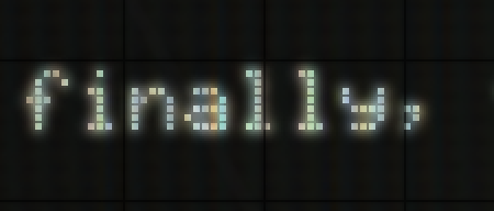
An LCD matrix font was used for the title text. This was just a PNG image of 128 characters that was spliced up and rearranged. This can be done in OpenCV by using submatrices and rectangle ROIs:
cv::Mat mat_font = cv::imread("lcd_font.png");
const cv::Size letter_size(24, 32);
const std::string text("finally, the end of the "
                       "marmalade forest!");

int cursor_x = 0;
for (char code : text_) {
  int mx = code % 32;
  int my = code / 32;

  cv::Rect font_roi(cv::Point(mx * letter_size.width,
                              my * letter_size.height),
                    letter_size);
  cv::Mat mat_letter = mat_font(font_roi);

  cv::Rect target_roi(text_origin_.x + cursor_x,
                      text_origin_.y,
                      mat_letter.cols, mat_letter.rows)
  mat_letter.copyTo(mat_output(target_roi));

  cursor_x += letter_size.width;
}
Encoding the video
Now we can save the frames as a video file. OpenCV has a VideoWriter class for just this purpose. But I like to do this a bit differently. I encoded the frame images individually as BMP and just concatenated them one after the other to stdout:
I then ran this program from a shell script that piped the output to ffmpeg for encoding. This way I could also combine it with the soundtrack in a single run.
A Finnish online bank used to include a US-based third-party analytics and tracking script in all of its pages. Ospi first wrote about it (in Finnish) in February 2015, and this caused a bit of a fuss.
The bank responded to users' worries by claiming that all information is collected anonymously:
But is it true?
As Ospi notes, a plethora of information is sent along the HTTP request for the tracker script. This includes, of course, the IP address of the user; but also the full URL the user is browsing. The bank's URLs reveal quite a bit about what the user is doing; for instance, a user planning to start a continuous savings contract will send the url continuousSavingsContractStep1.do.
I logged in to the bank (using well-known demo credentials) to record one such tracking request. The URL sent to the third party tracker contains a cleartext transaction archive code that could easily be used to match a transaction between two bank accounts, since it's identical for both users. But there's also a hex string called accountId (highlighted in red).
Remote Address: 80.***.***.***:443
Request URL:    https://www.google-analytics.com/collect?v=1&_v=j33&a=870588619&t
                =pageview&_s=1&dl=https%3A%2F%2Fonline.********.fi%2Febank%2Facco
                unt%2FinitTransactionDetails.do%3FbackLink%3Dreset%26accountId%3D
                69af881eca98b7042f18e975e00f9d49d5d5ee64%26rowNo%3D0%26type%3Dtra
                ns%26archivecode%3D20150220123456780002&ul=en-us&de=windows-1252&
                dt=Tilit%C2%A0%7C%C2%A0Verkkopankki%20%7C%20S-Pankki&sd=24-bit&sr
                =1440x900&vp=1440x150&je=1&fl=16.0%20r0&_u=QACAAQQBI~&jid=&cid=18
                39557247.1424801770&uid=&tid=UA-37407484-1&cd1=&cd2=demo_accounts
                &cd3=%2Ffi%2F&z=2098846672
Request Method: GET
Status Code:    200 OK
It's 40 hex characters long, which is 160 bits. This happens to be the length of an SHA-1 hash.
Could it really be a simple hash of the user's bank account number? Surely they would at least salt it.
Let's try!
The demo account's IBAN code is FI96 3939 0001 0006 03, but this doesn't give us the above hash. However, if we remove the country code, IBAN checksum, and all whitespaces, it turns out we have a match!
This is a BBAN format bank account number. BBAN numbers are easy to brute-force, especially if the bank is already known. I wrote the following C program, ~25 lines of code, that reversed the above hash to the correct account number in 0.5 seconds.
$ gcc -lcrypto -o bban_hash bban_hash.c

$ time ./bban_hash
found 39390001000603
./bban_hash  0.42s user 0.00s system 99% cpu 0.420 total

$ █
In conclusion, the third party is provided with the user's IP address, bank account number, addresses of subpages they visit, and account numbers associated with all transactions they make. The analytics company should also have no difficulty matching the user with its own database collected from other sites, including their full name and search history.
Incidentally, this is in breach of the Guidelines on bank secrecy (PDF) by the Federation of Finnish Financial Services; "In accordance with the secrecy obligation, third parties may not even be disclosed whether a certain person is a customer of the bank" (pg 4) (sama suomeksi: "Salassapitovelvollisuus sisältää myös sen, että sivullisille ei ilmoiteta edes sitä, onko tietty henkilö pankin asiakas vai ei").
Solution
The script was eventually removed from the site, leaving the bank regretful that such a useful tool was lost.
However, alternatives do exist (like Piwik) that can be run locally, not involving a third party. Edit:The Intercept, a news website, is using non-privacy-invading metrics.
One day you'll need to include real-time UTC timestamps in audio. It's useful when reconstructing events from long, unsupervised surveillance microphone recordings, or when constantly monitoring and logging radio channels.
There's no standard method for doing this with WAV or FLAC files. One method would be to log the start time in the filename and calculate the time based on audio position. However, this is not possible with voice-activated or squelched recorders. It also relies on the accuracy and stability of the ADC clock.
I'll take a look at some ways to include an accurate timestamp directly in the in-band audio.
Least significant bit
Time information can be encoded in the least significant bit (LSB) of the 16-bit PCM samples. This "steganographic" method requires a lossless file format and lossless conversions. The script below truncates all samples of a raw single-channel signed-integer PCM stream to 15 bits and inserts a 20-byte ISO 8601 timestamp in ASCII roughly every second, preceded by a "mark" start bit. When played back, the LSB can be zeroed out to get rid of the timestamps. The WAV can also be played as such; the "ticking" sound will be practically inaudible at an amplitude of −96 dB. The outgoing PCM stream is then sent to SoX for WAV encoding.
#!/usr/bin/perl
use strict;
use warnings;
use DateTime;

my $snum    = 0;
my $writing = 0;
my $pos     = 0;
my $code    = "";

open my $out, '-|', 'sox -t .raw -e unsigned-integer -b 16 -r 44100 '.
                    '-c 1 - stamped.wav';

while (read STDIN, my $sample, 2) {
  $sample = unpack "s", $sample;
  my $bit = 0;

  if ($writing) {
    $bit = (ord(substr $code, $pos >> 3, 1) >> ($pos % 8)) & 1;
    if (++$pos >= length $code << 3) {
      $writing = 0;
      $bit     = 0;
    }
  } elsif ($snum++ % 44100 == 0) {
    $writing = 1;
    $pos     = 0;
    $bit     = 1;
    $code    = DateTime->now()->iso8601();
  }

  print $out pack "S", ($sample + 0x7FFF) & 0xFFFE | $bit;

}
close $out;
Note that the start bit of the timestamp will mark the moment the sample reached this script, and it could differ hundreds of milliseconds from the actual moment of reception at the microphone. Also, the timestamp does not mark the start of a second, but is rather timed by an arbitrary sample counter. One could also poll and write the timestamps in a continuous manner.
The above script could be modified to interface with my squelch script, by only inserting timestamps when squelch is not active. The resulting audio could then be efficiently encoded as FLAC.
lsb-time-read.pl reads back the timestamps, also printing the sample position of each. Below is a sound sample of a clean signal followed by a timestamped one.
Lossy-friendly approach
Lossy compression, by definition, does not retain the numeric values of samples, so they can't be treated as bit fields. Instead, we can use an analog modulation scheme like binary FSK. MP3 and Ogg Vorbis encoders will, at a reasonable bit rate, retain the structure of a sufficiently slow FSK burst. This method will work even if the timestamping phase is followed by an analog conversion.
Using the ultrasonic part of the spectrum comes to mind; but unfortunately such high frequencies are mainly ignored by a LPF at the encoder. However, we can use the higher end of the remaining spectrum and filter it out afterwards, if the recording consists of narrow-band speech. In the case of squelched conversation, we could write the timestamp only in the beginning of each transmission. This way it could even be in the speech frequencies.
fsk-timestamp.pl embeds the timestamps into PCM data; they can be read back using minimodem --rx --mark 11000 --space 13000 --file stamped.wav -q 1200.