Passing planes and other whoosh sounds

I always assumed that the recognisable 'whoosh' sound a plane or helicopter makes when passing overhead simply comes from the famous Doppler effect. But when you listen closely, this explanation doesn't make complete sense.

(Audio clipped from freesound - here and here)

A classic example of the Doppler effect is the sound of a passing ambulance constantly descending in pitch. When a plane flies overhead the roar of the engine sometimes does that as well. But you can also hear a wider, breathier noise that does something different: it's like the pitch goes down at first, but when the plane has passed us, the pitch goes up again. That's not how Doppler works! What's going on there?

Comb filtering.

Let's shed light on the mystery by taking a look at the sound in a time-frequency spectrogram. Here, time runs from left to right, frequencies from top (high) to bottom (low).

We can clearly see one part of the sound (the one starting at 2500 Hz) sweeping downwards, or from high to low frequencies; this should be the Doppler effect. But there's something else happening at the bottom of the image – another pattern is moving down at first, then up again...

This sound's frequency distribution seems to form a series of moving peaks and valleys. This resembles what audio engineers would call 'comb filtering', due to its appearance in the spectrogram. When the peaks and valleys move about it causes a 'whoosh' sound; this is the same principle as in the flanger effect used in music production. But these are just jargon for the electronically created version. We can call the acoustic phenomenon the whoosh.

The comb pattern is caused by two copies of the same exact sound arriving at a slightly different times, close enough that they form an interference pattern. It's closely related to what happens to light in the double slit experiment. In recordings this often means that the sound was captured by two microphones and then mixed together; you can sometimes hear this happen unintentionally in podcasts and radio shows. So my thought process is, are we hearing two copies of the plane's sound? How much later is the other one arriving, and why? And why does the 'whoosh' appear to go down in pitch at first, then up again?

Into the cepstral domain.

The cepstrum, which is the inverse Fourier transform of the estimated log spectrum, is a fascinating plot for looking at delays and echoes in complex (as in complicated) signals. While the spectrum separates frequencies, the cepstrum measures time, or quefrency – see what they did there? It reveals cyclicities in the sound's structure even if it interferes with itself, like in our case. In that it's similar to autocorrelation.

It's also useful for looking at sounds that, experientially, have a 'pitch' to them but that don't show any clear spectral peak in the Fourier transform. Just like the sound we're interested in.

Here's a time-quefrency cepstrogram of the same sound (to be accurate, I used the autocepstrum here for better clarity):

The Doppler effect is less prominent here. Instead, the plot shows a sweeping peak that seems to agree with the pitch change we hear. This delay time sweeps from around 4 milliseconds to 9 ms and back. Note that the scale: higher frequencies (shorter times) are on the bottom this time.

Now why would the sound be so correlated with itself with this sweeping delay time?

Ground echo?

Here's my hypothesis. We are hearing not only the direct sound from the plane but also a delayed echo from a nearby flat surface. These two sound get superimposed and interfere before they reach our ears. The effect would be especially prominent with planes and helicopters because there is little in the way of the sound either from above or from the large surface. And what could be a large reflective surface outdoors? Well, the ground below!

Let's think about the numbers. The ground is around one-and-a-half metres below our ears. When a plane is directly overhead, the reflected sound needs to take a path that's three metres longer (two-way) than the direct path. Since sound travels 343 metres per second this translates to a difference of 9 milliseconds – just what we saw in the correlogram!

Below, I used GeoGebra to calculate the time difference (between the yellow and green paths) in milliseconds.

When the plane is far away the angle is shallower, the two paths are more similar in distance, and the time difference is shorter.

It would follow that a taller person hears the sound differently than a shorter one, or someone in a tenth-floor window! If the ground is very soft, maybe in a mossy grove, you probably wouldn't hear the effect at all; just the Doppler effect. But this prediction needs to be tested out in a real forest.

Here's what a minimal acoustic simulation model renders. We'll just put a flying white noise source in the sky and a reflective surface as the ground. Let's only update the IR at 15 fps to prevent the Doppler phenomenon from emerging.

Whoosh!

Some everyday whooshes.

The whoosh isn't only associated with planes. When it occurs naturally it usually needs three things:

  • a sound with a lot of structure (preferably a hissy or breathy noise)
  • an unobstructed echo from a closeby surface
  • and some kind of physical movement.

I've heard this outdoors when the sound of a waterfall was reflecting off a brick wall (video); and next to a motorway when the sound barrier provided the reflection. You can hear it in some films – for instance, in the original Home Alone when Kevin puts down the pizza box after taking a whiff (video)!

You can even hear it in the sound of thunder when lightning hits quite close. Nothing is physically moving in this case; but it might be caused because a 'bang' is created simultaneously along a very long path but sound only travels so fast.

Try it yourself: move your head towards a wall – or a laptop screen – and back away from it, while making a continuous 'hhhh' or 'shhh' noise. Listen closely but don't close your eyes, you might bump your nose.

Where have you encountered the whoosh?

A simple little plot.

Finally, if you have JavaScript turned on you'll see (and hear) some more stuff in this blog post. In the interactive graph below you can move the aeroplane and listener around and see how the numbers change. The 'lag' or time difference we hear (orange arrow) comes from how much farther away the reflected virtual image is compared to the real aeroplane. For instance, when it's right above, the copied sound travels 3 meters longer. In the lower right corner, the 'filter' spectrum up to 4.5 kHz is also drawn. The circles are there to visualize the direct distance.

FAQ

I get many questions that point out that planes have two of something: two engines, two ends in one engine, etc... I can see how this is an inviting chain of though, but it has two problems. 1) The sound is not just associated to jet engines or even planes at all; 2) The sounds would have to be nearly identical for interference to happen. Random wind noise wouldn't created phase-coherent sounds from two independent sources. Some discussion in the comments below.

Ultrasonic investigations in shopping centres

I can't remember how I first came across these near-ultrasonic 'beacons' ubiquitous in PA systems. I might have been scrolling through the audio spectrum while waiting for the underground train; or it might have been the screeching 'tinnitus-like' sensation I would often get near the loudspeakers at a local shopping centre.

[Image: Graph with frequencies from 16 to 24 kHz and decibels from -30 to -110. Two peaks are shown, the lower one marked REDI around 19600 Hz and a higher one marked Forum at 20000 Hz.]

Whatever the case, I learned that they are called pilot tones. Many multi-loudspeaker PA systems (like the Zenitel VPA and Axys End of Line detection unit) employ these roughly 20-kilohertz tones to continuously measure the system's health status: no pilot tone means no connection to a loudspeaker. It's usually set to a very high frequency, inaudible to humans, to avoid disturbing customers.

However, these tones are powerful and some people will still hear them, especially if the frequency gets below 20 kHz. There is one such system at an uncomfortable 19.595 kHz in my city; it's marked green in the graph above. I've heard of several other people that also hear the sound. I don't believe it to be a sonic weapon like The Mosquito; those use even lower frequencies, down to 17 kHz. It's probably just a misconfiguration that was never fixed because the people working on it couldn't experientially confirm any issue with it.

Hidden modulation.

Pretty quickly it became apparent that this sound is almost never a pure tone. Some kind of modulation can always be seen wiggling around it in the spectrogram. Is it caused by the background music being played through the PA system? Is it carrying some information? Or is it something else altogether?

I've found at least one place where the tone appears to be amplitude modulated by the lowest frequencies in the music or commercials playing. It's probably a side effect of some kind of distortion.

Here's a spectrogram plot of this amplitude modulation around the strong pilot tone. It's colour-coded so that the purple colour is coming from the right microphone channel and green from the left. I'm not quite sure what the other purple horizontal stripes are here.

But this kind of modulation is rare. It's more common to see the tone change in response to things happening around you, like people moving about. More on that in the following.

Doppler-shifted backscatter.

Look what happens to the pilot tone when a train arrives at an underground station:

The wideband screech in the beginning is followed by this interesting tornado-shaped pattern that seems to have a lot of structure inside of it. It lasts for 15 seconds, until the train comes to a stop.

It's my belief that this is backscatter, also known as reverb, from the pilot tone reflecting off the slowing train and getting Doppler-shifted on the way. The pilot tone works as a continuous-wave bistatic sonar. Here, the left microphone (green) hears a mostly negative Doppler shift whereas the right channel (purple) hears a positive one, as the train is passing us from right to left. An anti-aliasing filter has darkened the higher frequencies as I wasn't yet aware I would find something interesting up here when recording.

A zoomed-in view of this cone reveals these repeating sweeps from positive to negative and red to green. Are they reflections off of some repeating structure in the passing train? The short horizontal bursts of constant tone could then be surfaces that are angled in a different direction than the rest of the train. Or perhaps this repetition reflects the regular placement of loudspeakers around the station?

Moving the microphone.

Another interesting experiment: I took the lift to another floor and recorded the ride from inside the lift. It wasn't the metal box type, the walls were made of glass, so I thought the pilot tone should be at least somewhat audible inside. Here's what I got during the 10-second ride. It's a little buried in noise.

[Image: A spectrogram zoomed into 19500 Hz. There's a pure tone at 19500 Hz in the beginning. Soon it starts to 'disintegrate' into wideband noise and then comes back together, forming a spindle-like pattern.]

Skater calculation.

For the next experiment I went into the underground car park of a shopping centre. I stood right under a PA loudspeaker and recorded a skateboarder passing by. A lot of interesting stuff is happening in this stereo spectrogram!

[Image: A pure tone near 19500 Hz, superimposed with an S-shaped pattern going from higher to lower frequencies and from red to green colour.]

First of all, there seems to be two pilot tones, one at 19,595 Hz and a much quieter one at 19,500 Hz. Are there two different PA systems in the car park?

Second, there's a clear Doppler shift in the reverb. The frequency shift goes from positive to negative at the same moment that the skater passes us, seen as the wideband wheel noise changing color. It looks like the pattern is also 'filled in' with noise under this Doppler curve. What all information can we find out just by looking at this image?

If we ignore the fact that this is actually a bistatic doppler shift we could try and estimate the speed using a formula on Wikipedia. It was pretty chilly in the car park, I would say 15 °C. The speed of sound at 15 °C is 340 m/s. The maximum Doppler shift here seems to be 350 Hz. Plugging all these into the equation we get 11 km/h, which sounds like a realistic speed for a skater.

Why is it filled in? My thought is these are reflections off different points on our test subject. There's variation in the reflection angles and, consequently, magnitudes of the velocity component that causes frequency shifting, down to nearly zero Hz.

What now?

What would you do with this ultrasonic beep all around you? I have some free ideas:

  • Automated speed trap in the car park
  • Detect when the escalators stop working
  • Modulate it with a positioning code to prevent people getting lost in the maze of commerce
  • Use it to deliver ads somehow
  • Use it to find your way to the quietest spots in a shopping centre

Smoother sailing: Studying audio imperfections in Steamboat Willie

[Image: Mickey Mouse whistling on the bridge of a steamboat.]

Steamboat Willie (1928) was one of the earliest cartoons with synchronized sound. That is, it had post-production sound effects; this was something new and exciting. Now that the cartoon has recently entered the public domain[bbc24] we can safely delve into its famous soundtrack. See, there's something interesting about how it sounds...

If you listen closely to the soundtrack on Youtube it sounds somehow distorted. You might be tempted to point out that it's 96 years old, yes. But you might also recognize that it is suffering from flutter, i.e. an unstable playback or recording speed.

In the spirit of this blog let's geek out for a bit and study this flutter distortion further. Can we learn something interesting? Could we perhaps learn enough to be able to reduce it?

Of course the flutter might be 100% authentic to how it sounded in theatres in the 1920s; we don't know when and why it appeared in the audio (more on that later!). It might have sounded even worse. But we can still hope to enjoy the sound effects in their original recorded form.

Prior work

I'm not the first one to notice this clip is 'fluttering' and to try and do something about it. I found videos of people's attempts to un-flutter it using Celemony Capstan, a professional tool made just for this purpose, with varying results. Capstan uses Melodyne's famous note detection engine to detect musical features and then controls a varispeed effect to cancel out any flutter.

But Capstan is expensive, and it's more fun to come up with a home-made solution anyway. And what about non-musical sounds? Besides, I had some code laying around in a forgotten desk drawer that just might fit the purpose.

Finding a high quality source

Why would I need a high-quality digital file of a poor-quality soundtrack from the 1920s? I guess it's the archivist in me hoping that it has been preserved with high level of detail. But also, if you're going to try and dig up some hidden details in the sound, you'd want minimal interference from any lossy psychoacoustic compression, right? These artifacts might become audible after varispeed effects and could also hinder frequency detection.

[Image: Two spectrograms labeled 'random Youtube video' and '4K version', the former showing compression artifacts.]

The high-quality source I found is in the Internet Archive. It might originally be coming from the 4K Blu-Ray release called Celebrating Mickey. The spectrogram doesn't show almost any compression artifacts that I can see, even in the quietest frequency ranges! Perfect!

[Image: A single film frame.]

But the Internet Archive delivers something even better. There's a (visually) lossless 4K scan of the movie with the optical soundtrack partially included (above)! The high-quality version is 34 GB, but there's a downscaled 480p MP4 one thousandth of the size.

I listened to the optical soundtrack from this low-resolution version with a little pixel-reader script. Turns out the flutter is already present on the film! (Edit: Note that we don't know where this particular film print came from. When was it created? Is there an original somewhere, without flutter?)

Hand-guiding a frequency tracker

Looking at the above spectrogram, we can see that the frequency of everything is zig-zagging as a function of time – that's flutter all right. But how to quantify these variations? We could zoom in on one of the frequency peaks and follow the course of its frequency in time. I'm using FFT peak interpolation to find more accurate frequency estimates[gasior04].

Take the sound of Pete's tobacco hitting the ship's bell around the 01'45'' mark. You'd think a bell is supposed to have a constant frequency, yet this one sounds quite unstable. We can follow any one of the harmonics and see how the playback speed (bell frequency) varies over the period of one second:

[Image: Spectrogram with fluctuating tones.]

To my eye, this oscillation looks periodic and not random at all. We can run another round of FFT on a longer stretch of samples to find the strongest period of these fluctuations: It turns out to be 15 Hz. (Why 15? I so hoped it would have been 24 Hz – it would have made a more interesting story! More on that later...)

[Image: Spectrum plot showing a peak at 15.0 Hz about 15 dB higher than background.]

Okay, so can we repeat this process for the whole movie? I don't think we can just automatically follow the frequency of every peak, since some sounds will naturally contain vibration and rises and drops in frequency. Not all of it is due to flutter. Some sort of a vetting process is needed. We could try a tedious manual route...

[Image: GUI of a software with spectrograms and oscillogram plots.]

I made a little software tool (above) where I could click and drag little boxes onto a spectrogram to search for peaks in. This wobbly line is then simply taken to be the speed variation (red graph in the top picture).

It became quite a chore to annotate longer sounds as this software didn't come with undo, edit, or save features for the longest time!

Now let's think about what to do with this speed information...

Desk drawer deep dive

Some time ago I had made a tool that could well come in handy now. It was for correcting wobbly wideband radio recordings stored on VHS tapes. These recordings contained some empty carriers that happened to work like seismographs, accurately recording the tape speed variations. The tool then used a Lagrange polynomial to interpolate new samples at a steady interval, so called 'digital varispeed'.

It was ultimately based on an interesting paper on de-fluttering magnetic tapes using the tape bias signal as reference[howarth04].

[Image: Buttons of an old device, one of them Varispeed, labeled 1981. Below, part of a GUI with the text Varispeed, labeled 2023.]

By the way, I keep mentioning varispeed and never explained it. This was a feature of old studio-grade reel-to-reel tape recorders where the playback speed could be freely varied by the operator; hence vari+speed. Audio people still use this word in the digital world to essentially refer to variable-rate resampling, which has the same effect, so I'm using them interchangeably. (Topmost photo: Ferdinando Traversa, CC BY, cropped to detail)

Here's what this digital varispeed sounds like when exaggerated. In the below example I'm doing it in a simpler way. Instead of the Lagrange method I first upsampled some music by 10x in an audio software; hand-drew a speed curve in Audacity; and then used that curve to pick samples out of the oversampled music:

[Image: A waveform in Audacity.]

Carefully controlled, this effect can be used to cancel out flutter. Here's how: If we knew exactly how the playback speed was fluctuating we could instantly vary the speed of our resampler in the opposite direction, thus canceling the variations. And with the above research we now have that knowledge!

Well, almost. I couldn't always see a clear frequency peak to follow, so the graph is patchy. But.. Maybe it could help to band-pass the speed signal at 15 Hz? This would help fill out small gaps and also preserve vibrato and other fluctuations that aren't part of the flutter distortion. We can at least try!

[Image: Two waveforms, one of them piecewise and noisy, the other one smooth and continuous.]

In the example above, I replaced empty parts with a constant value of 100% and then filtered the whole thing. This sews the disjointed parts together in a smooth way.

Can we hear some examples already?

This clip is from when the goat ate Minnie's sheet music and guitar – the apparent catalyst event that sent Mickey Mouse to seek revenge on the entire animal kingdom.

You can definitely hear the difference in the bell-like sounds coming from the goats insides. It even sounds like the little flute notes in the beginning are easier to tell apart in the corrected version.

Here's another musical example, with strings.

The cow's moo. That's a hard one because it's so rich in harmonics, in the spectrogram it looks almost like a spaghetti bolognese. My algorithm is constrained to a box and can't stay with one harmonic when the 'moo' slides in frequency. You can hear some artifacts because of this, but still the result sounds less sheep-like than the original.

Before [Image: Movie screenshot]
After

But Mickey whistling "Steamboat Bill" in the beginning of the film actually doesn't sound better when corrected... I preferred a bit of vibrato!

Before [Image: Movie screenshot]
After

Sidetrack 1: Anything else we can find?

Glad you're still reading! Let's step away from flutter for a while and take the raw audio track itself under the Fourier microscope. Zooming closer, is there anything interesting in the lower end?

[Image: Spectrogram showing a frequency range from 0 to 180 Hz.]

We can faintly see peaks at multiples of both 24 and 60 Hz. No surprises there, really... 24 Hz being the film framerate and 60 Hz the North American mains frequency. Was there a projector running in the recording studio? Or maybe it's an artifact of scanning the soundtrack one frame at a time? In any case, these sounds are pretty weak.

[Image: Spectrogram showing tones with apparent sidebands.]

In some places you can see some sort of modulation that seems to be generating sidebands, just like in radio signals. It's especially visible in Mickey's whistle when it's flutter-corrected, here at the 5-second mark. The sidebands peaks are 107 and 196 Hz away from the 'carrier' if you will. I'm not sure what this could be. Fluctuating amplitude?

Sidetrack 2: Playing sound-on-film frame by frame?

This is an experiment I did some time ago. It's just a silly thought - what would happen if the soundtrack was being read in the same way as the picture is – stopped 24 times per second? Would this be the ultimate flutter distortion?

In the olden days, sound was stored on the film next to the picture frames as analog information. Unlike the picture frames that had to be stopped momentarily for projection, the sound had to be played at a constant speed. There was a complicated mechanism in the projector to make this possible.

I found some speed curves for old-school movie projectors in [bickford72]. They describe the film's deceleration and acceleration during these stops. Let's emulate these speed curves in audio with the oversampling varispeed method.

The video below is a 3D animation where this same speed curve controls an animation of a moving film in an imaginary machine. The clip is from another 1920s animation, Alice in the Wooly West (1926).

~~ Now we know ~~

Conclusions

  • We found a 15 Hz speed fluctuation that was, to some extent, reversible.
  • This flutter signal is already present in the optical soundtrack of a film scan (of unknown origin).
  • With enough manual work, much of the soundtrack could probably be 'corrected'.
  • 'Hmm, that sounds odd' are sometimes the words of a white rabbit.

References

Using HDMI EMI for fast wireless data transfer

This story, too, begins with noise. I was browsing the radio waves with a software radio, looking for mysteries to accompany my ginger tea. I had started to notice a wide-band spiky signal on a number of frequencies that only seemed to appear indoors. Some sort of interference from electronic devices, probably. Spoiler alert, it eventually led me to broadcast a webcam picture over the radio waves... but how?

It sounds like video

The mystery deepened when I listened to how this interference sounded like as an AM signal. It reminded me of a time I mistakenly plugged our home stereo system to the Nintendo console's video output and heard a very similar buzz.

Am I possibly listening to video? Why would there be analog video transmitting on any frequency, let alone inside my home?

[Image: Oscillogram of a noisy waveform that seems to have a pulse every 10 microseconds or so.]

If we plot the signal's amplitude against time we can see that there is a strong pulse exactly 60 times per second. This could be the vertical synchronisation signal of 60 Hz video. A shorter pulse (pictured above) can be seen repeating more frequently; it could be the horizontal one. Between these pulses there is what appears to be noise. Maybe, if we use the strong pulses for synchronisation and plot the amplitude of that noise as a two-dimensional picture, we could see something?

And sure enough, when main screen turn on, we get signal:

[Image: A grainy greyscale image of what appears to be a computer desktop.]

(I've hidden the bright synchronisation signal from this picture.)

It seems to be my Raspberry Pi's desktop with weirdly distorted greyscale colours! Somehow, some part of the monitor setup is radiating it quite loudly into the aether. The frequency I'm listening to is a multiple of the monitor's pixel clock frequency.

As it turns out, this vulnerability of some monitors has been known for a long time. In 1985, van Eck demonstrated how CRT monitors can be spied on from a distance[1]; and in 2004, Markus Kuhn showed that the same still works on flat-screen monitors[2]. The image is heavily distorted, but some shapes and even bigger text can be recognisable. Sometimes this kind of eavesdropping is called "van Eck phreaking", in reference to phone phreaking.

The next thought was, could we get any more information out of these images? Is there any information about colour?

Mapping all the colours

HDMI is fully digital; there is no linear dependency between pixel values and greyscale brightness in this amplitude image. I believe the brightness in the above image is related to the number of bit transitions over my radio's sampling time (which is around 8 bit-lengths); and in HDMI, this is dependent on many things, not just the actual RGB value of the pixel. HDMI also uses multiple differential wires that all are transmitting their own picture channels side by side.

This is why I don't think it's possible easy to reconstruct a clear picture of what's being shown on the screen, let alone decode any colours.

But could the reverse be possible? Could we control this phenomenon to draw the greyscale pictures of our choice on the receiver's screen? How about sending binary data by displaying alternating pixel values on the monitor?

[Image: On the left, gradients of red, green, and blue; on the right, greyscale lines of seemingly unrelated brightness.]

My monitor uses 16-bit colours. There are "only" 65,536 different colours, so it's possible to go through all of them and see how each appears in the receiver. But it's not that simple; the bit-pattern of a HDMI pixel can actually get modified based on what came before it. And my radio isn't fast enough to even tell the bits apart anyway. What we could do is fill entire lines with one colour and average the received signal strength. We would then get a mapping for single-colour horizontal streaks (above). Assuming a long run of the same colour always produces the same bitstream, this could be good enough.

[Image: An XY plot where x goes from 0 to 65536 and Y from 0 to 1.2. A pattern seems to repeat itself every 256 values of x. Values from 16128 to 16384 are markedly higher.]

Here's the map of all the colours and their intensity in the radio receiver. (Whatever happens between 16,128 and 16,384? I don't know.)

Now, we can resample a greyscale image so that its pixels become short horizontal lines. Then, for every greyscale value find the closest matching RGB565 color in the above map. When we display this psychedelic hodge-podge of colour on the screen (on the right), enough of the above mapping seems to be preserved to produce a recognizable picture of a movie[3] on the receiver side (on the left):

[Image: On the right, a monitor shows a noisy green and blue image. On the left, another monitor shows a grainy picture of a man and the text 'Hackerman'.]

These colours are not constant in any way. If I move the antenna around, even if I turn it from vertical to horizontal, the greyscales will shift or even get inverted. If I tune the radio to another harmonic of the pixel clock frequency, the image seems to break down completely. (Are there more secrets to be unfolded in these variations?)

The binary exfiltration protocol

Now we should have enough information to be able to transmit bits. Maybe even big files and streaming data, depending on the bitrate we can achieve.

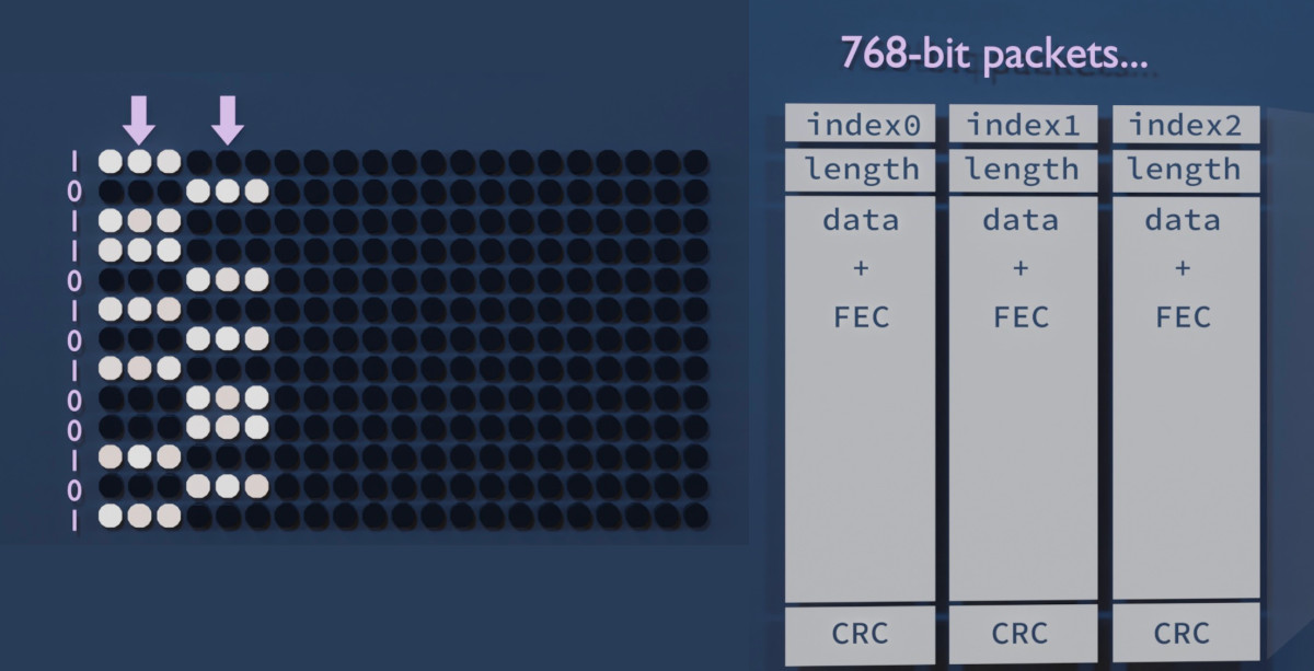
First of all, how should one bit be encoded? The absolute brightness will fluctuate depending on radio conditions. So I decided to encode bits as the brightness difference between two short horizontal lines. Positive difference means 1 and negative 0. This should stay fairly constant, unless the colours completely flip around that is.

[Image: When a bit is 0, the leftmost line is darker than the rightmost line, and vice versa. These lines are used to form 768-bit packets.]

The monitor has 768 pixels vertically. This is a nice number so I designed a packet that runs vertically across the display. (This proved to be a bad decision, as we will later see.) We can stack as many packets side-by-side as the monitor width allows. A new batch of packets can be displayed in each frame, or we can repeat them over multiple frames to improve reliability.

These packets should have some metadata, at least a sequence number. Our medium is also quite noisy, so we need some kind of forward error correction. I'm using a Hamming(12,8) code which adds 4 error correction bits for every 8 bits of data. Finally, we need to add a CRC to each packet so we can make sure it arrived intact; I chose CRC16 with the polynomial 0x8005 (just because liquid-dsp provided it by default).

First results!

It was quite unbelievable, I was able to transmit a looping 64 kbps audio stream almost without any glitches, with the monitor and the receiver in the same room approximately 2 meters from each other.

Quick tip. Raw 8-bit PCM audio is a nice test format for these kinds of streaming experiments. It's straightforward to set an arbitrary bitrate by resampling the sound (with SoX for instance); there's no structure, headers, or byte order to deal with; and any packet loss, misorder, or buffer underrun is instantly audible. You can use a headerless companding algorithm like A-law to fit more dynamic range in 8 bits. Even stereo works; if you start from the wrong byte the channels will just get swapped. SoX can also play back the stream.

But can we get more? Slowly I added more samples per second, and a second audio channel. Suddenly we were at 256 kbps and still running smoothly. 200 kbps was even possible from the adjacent room, with a directional antenna 5 meters away, and with the door closed! In the same room, it worked up to around 512 kilobits per second but then hit a wall.

[Image: Info window that says HasPreamble: 1. Total: 928.5 kbps, Fresh: 853.6 kbps, Fresh (payload): 515.7 kbps.]

A tearful performance

The heavy error correction and framing adds around 60% of overhead, and we're left wit 480 bits of 'payload' per packet. If we have 39 packets per frame at 60 frames per second we should get more than a megabit per second, right? But for some reason it always caps at half a megabit.

The reason revealed itself when I noticed every other frame was often completely discarded at the CRC check. Of course; I should have thought of properly synchronising the screen update to the graphics adapter's frame update cycle (or VSYNC). This would prevent the picture information changing mid-frame, also known as tearing. But whatever options I tried with the SDL library I couldn't get the Raspberry Pi 4 to not introduce tearing.

Screen tearing appears to be an unsolved problem plaguing the Raspberry Pi 4 specifically (see this Google search). I tried another mini computer, the Asus Tinker Board R2.0, but I couldn't get the graphics drivers to work properly. I then realised it was a mistake to have the packets run from top to bottom; any horizontal tearing will cut every single packet in half! With a horizontal design only one packet per frame would suffer this fate.

A new design enables video-over-video

Packets that run horizontally across the screen indeed fix most of the packet loss. It may also help with CPU load as it improves memory access locality. I'm now able to get 1000 kbps from the monitor! What could this be used for? A live video stream, perhaps?

But the clock was ticking. I had a presentation coming up and I really wanted to amaze everyone with a video transfer demo. I quite literally got it working on the morning of the event. For simplicity, I decided to go with MJPEG, even though fancier schemes could compress way more efficiently. The packet loss issues are mostly kept at bay by repeating frames.

The data stream is "hidden" in a Windows desktop screenshot; I'm changing the colours in a way that both creates a readable bit and also looks inconspicuous when you look from far away.

Mitigations

This was a fun project but this kind of a vulnerability could, in the tinfoiliest of situations, be used for exfiltrating information out of a supposedly airgapped computer.

The issue has been alleviated in some modern display protocols. DisplayPort[4] makes use of scrambling: a pseudorandom sequence of bits is mixed with the bitstream to remove the strong clock oscillations that are so easily radiated out. This also randomizes the bitstream-to-amplitude correlation. I haven't personally tested whether it still has some kind of video in their radio interference, though. (Edit: Scrambling seems to be optionally supported by later versions of HDMI, too – but it might depend on which features exactly the two devices negotiate. How could you know if it's turned on?)

[Image: A monitor completely wrapped in tinfoil, with the text IMPRACTICAL written over it.]

I've also tried wrapping the monitor in tinfoil (very impractical) and inside a cage made out of chicken wire (it had no effect - perhaps I should have grounded it?). I can't recommend either of these.

Software considerations

This project was made possible by at least C++, Perl, SoX, ImageMagick, liquid-dsp, Dear Imgui, GLFW, turbojpeg, and v4l2! If you're a library that feels left out, please leave a comment.

If you wish to play around with video emanations, I heard there is a project called TempestSDR. For generic analog video decoding via a software radio, there is TVSharp.

References

  1. Van Eck, Wim (1985): Electromagnetic radiation from video display units: An eavesdropping risk?
  2. Kuhn, Markus (2004): Electromagnetic Eavesdropping Risks of Flat-Panel Displays
  3. KUNG FURY Official Movie [HD] (2015)
  4. Video Electronics Standards Association (2006): DisplayPort Standard, version 1.

Spiral spectrograms and intonation illustrations

I've been experimenting with methods for visualising harmony, intonation (tuning), and overtones in music. Ordinary spectrograms aren't very well suited for that as the harmonic relations are not intuitively visible. Let's see what could be done about this. I'll try to sprinkle the text with Wikipedia links in order to immerse (nerd snipe?) the reader in the subject.

Equal temperament cents against time

We can examine how tuning evolves during a recording by choosing a reference pitch and plotting all frequencies relative to it modulo 100 cents. This is similar to what an electronic tuner does, but instead of just showing the fundamental frequency, we'll plot the whole spectrum. Information about the absolute frequencies is lost. This "zoomed-in" plot visualises how the distribution of frequencies fits the 12-tone equal temperament system (12-TET) common in Western music.

Here's the first 20 seconds of Debussy's Clair De Lune as found on YouTube, played with a well-tuned (video) and an out-of-tune piano (video). The second piano sounds out of tune because there are relative differences in tuning between the strings. The first piano looks to be a few cents sharp as a whole, but consistently so, so it's not perceptible.

[Image: Two spectrograms labeled 'Piano in tune' and 'Piano out of tune'. The first one shows blobs of light along the center axis. In the second one, the blobs are jumping up and down the graph.]

The vertical axis is the same that electronic tuners use. All the notes of a chord will appear in the middle, as long as they are well tuned against the reference pitch of, say, A = 440 Hz. The top edge of the graph is half a semitone sharp (quarter tone = 50c), and the bottom is half a semitone flat.

Overtones barely appear in the picture because the first three conveniently hit other notes in tune. But from f5 onwards the harmonic series starts deviating from 12-TET and the harmonics start to look out-of-tune (f5 = −14c, f7 = −31c, ...). These can be cut out by filtering, or hoping that they're lower in volume and setting the color range accordingly.

Six months later...

You know how you sometimes accidentally delete a project and have to rewrite it from scratch much later, and it's never exactly the same? That's what happened at this point. It's a little scuffed, but here's some piano music that utilises quarter tones (by Wyschnegradsky). I used the same scale on purpose, so the quarter tones wrap around from the top and bottom.

[Image: Similar as above, but blobs are also seen at the very top and bottom of the graph.]

More examples of these "intonation plots" in a tweet.

This suits well for piano music. However, not even all western classical music is tuned to equal temperament; for instance, solo strings may be played with Pythagorean intonation[1], whereas vocal ensembles[2] and string quartets may tune some intervals closer to just intonation. Unlike the piano, these wouldn't look too good in the equal-note plot.

Octave spiral

If we instead plot the spectrum modulo 1200 cents (1 octave) we get an interesting interval view. We could even ditch the time scale and wind the spectrogram into a spiral to make it prettier and preserve the overtones and absolute frequency information. Now each note is represented by an angle in this spiral; in 12-TET, they're separated by 30 degrees. At any point in the spiral, going 1 turn outwards doubles the frequency.

Here's a C major chord on a piano. Note how the harmonic content adds several high-frequency notes on top of the C, E, and G of the triad chord, and how multiple notes can contribute to the same overtone:

[Image: 12 note names labeled around a spiral. The C, E, and G notes light up sequentially, and their frequency and harmonics are displayed on the spiral.]

I had actually hoped I would get an Ultimate Chord Viewer where any note, regardless of frequency, would have all its harmonics neatly stacked on top of it. But it's not what has happened here: the harmonic series is not a stack of octaves (2^n), but instead of integer multiples (n). Some harmonics appear at seemingly unrelated angles. But it's still a pretty interesting visualisation, and perhaps makes more sense musically.

This plot is also better at illustrating different tuning systems. Let's look at a major third interval F-A in equal temperament and just intonation, with a few more harmonics.

[Image: The interval alternates between 400 and 386 cents. When it's 386, a few harmonics of the F note merge with those of the A note.]

The intuition from this plot is that equal temperament aims for equal distances (angles) between notes and just intonation tries to make more of the harmonics match instead.

Even though the Ultimate Chord Viewer was not achieved I now have ideas for Christmas lights...

Live visualization

Here's what a cappella music with some reverb looks like on the spiral spectrogram.

A shader toy

This little real-time GLSL demo on shadertoy draws a spiral FFT from microphone audio. But don't get your hopes up: The spectrograms in this blog post were made with a 65536-point FFT. Shadertoy's 512px microphone texture offers a lot less in terms of frequency range and bins. This greatly blurs the frequency resolution, especially towars the low end. Could it be improved with the right colormap? Or a custom FFT with the waveform texture as its input?

References

Speech to birdsong conversion

I had a dream one night where a blackbird was talking in human language. When I woke up there was actually a blackbird singing outside the window. Its inflections were curiously speech-like. The dreaming mind only needed to imagine a bunch of additional harmonics to form phonemes and words. One was left wondering if speech could be transformed into a blackbird song by isolating one of the harmonics...

One way to do this would be to:

  • Find the instantaneous fundamental frequency and amplitude of the speech. For example, filter the harmonics out and use an FM demodulator to find the frequency. Then find the signal envelope amplitude by AM demodulation.
  • Generate a new wave with similar amplitude variations but greatly multiplied in frequency.
[Image: Signal path diagram.]

A proof-of-concept script using the Perl-SoX-csdr command-line toolchain is available (source code here). The result sounds surprisingly blackbird-like. Even the little trills are there, probably as a result of FM noise or maybe vocal fry at the end of sentences. I got the best results by speaking slowly and using exaggerated inflection.

Someone hinted that the type of intonation used in certain automatic announcements is perfect for this kind of conversion. And it seems to be true! Here, a noise gate and reverb has been added to the result to improve it a little:

And finally, a piece of sound art where this synthetic blackbird song is mixed with a subtle chord and a forest ambience:

Think of the possibilities: A simultaneous interpreter for talking to birds. A tool for dubbing talking birds in animation or live theatre. Entertainment for cats.

What other birds could be done with a voice changer like this? What about croaky birds like a duck or a crow?

(I talked about this blog post a little on NPR: Here's What 'All Things Considered' Sounds Like — In Blackbird Song)

Plotting patterns in music with a fantasy record player

[Image: Close-up of a vinyl record showing a wavy pattern.]

Back in April I bought a vinyl record that had a weird wavy pattern near the outer edge. I though I may have broken it somehow but couldn't even test this because I don't own a record player. *) But when I took a closer look at the pattern it seemed to somehow follow changes in the music. That doesn't look like damage at all.

When I played the CD version it became clear: this was an artifact of the tempo of the electronic track (100 bpm) being a multiple of the rotational speed (33 1/3 rpm), and these were probably drum hits! My tweet sparked some interesting discussion and I've been pondering this ever since. Could we plot any song as a loop or grid based on its own tempo and see interesting patterns?

(*) I know, it's a little odd. But I have a few unplayed vinyl records waiting for the day that I finally have the proper equipment. By the way, the song was Black Pink by RinneRadio from their wonderful album staRRk.

I wrote a little script to do just this: to plot the amplitude of the FLAC into a grid with an adjustable width. The result looks very similar to the pattern on the vinyl surface! Note that this image is a "straightened out" version of the disc surface and it's showing three of those wavy patterns. The top edge corresponds to the outer edge of the vinyl.

[Image: A plot showing similar patterns that were on the disc surface.]

Later I wrote a little more ambitious plotter that shall be explained soon.

Computer-conducted music gives best patterns

After plotting several different songs against their own tempo like this it seemed that in addition to electronic music a lot of pop and rock has this type of a pattern, too. The most striking and clear patterns can be seen in music that makes use of drum samples in a quantized time base (aka. a drum machine): the same kick drum sample, for example, repeats four times in each bar, perfectly timed by a computer so that they align in phase.

Somewhat similar patterns can be seen in live music that is played to a "click track": each band member hears a common computer-generated time signal in their earplug so that they won't sway from an average tempo. But of course the live beats won't be perfectly phase-aligned in this case, because the musicians are humans and there's also physics involved.

3D rendered video experiment

To demonstrate how the patterns on vinyl records are born I made a video showing a fantasy record player that can play an "e-ink powered optical record" and morph it into any RPM. I say fantasy because it's just that: imagination, science fiction, rendered 3D art - it would be quite unfeasible in real life. You can't actually make e-ink displays that fast and accurate. But of course it would be possible to have a live display of a digitally sampled audio file as a spiral and use some kind of physical controllers to change the RPM value in real time, and just play the sound from a digital file.

Making the video was really fun and I think the end result is equal parts weird and illustrating.

Programming the disk surface and audio

The disc surface is based on a video texture: a different image was rendered for each changed frame using a purpose-written C++ program. The program uses an oversampled (8x) version of the original music that it then resamples at a variable rate based on the recorded RPM value (let's call it a morphing value). Oversampling and low-pass filtering beforehand makes variable-rate resampling simple: just take a sample at the appropriate time instant and don't worry about interpolation. It won't sound perfect but actually the artifact adds an interesting distortion, perhaps simulating pixel boundaries in the 'e-ink display'.

The amplitude sample at each time instant was projected into polar coordinates and plotted as an image. The image is fairly large - at least 2048 by 2048 pixels. I use this as a sort of image-space oversampling to get the polar projection to look a little better. I even tried 8192 x 8192 video but it was getting too heavy on my computer. But a new image must only be generated when the morphing value changes; the other frames can be copied.

[Image: A square image of the disc video texture.]

The sound track was made by continuously sampling the position of the "play head" 44100 times per second, whether the disk was moving or not. Which sample ends up in the audio depends on the current rotational angle and the morphing value of the disk surface. When either of those values change it moves the audio past the play head. A DC cancel filter was then applied because the play head would often stop on a non-zero sample, and it didn't look nice in the waveform. There's also a quiet hum in the background.

[Image: Screenshot of C++ code with a list of events.]

I made an event-based system where I could input events simulating the button presses and other controls. The system responds to speed change events with a smoothstep function so that the disc seems to have realistic inertia. Also, the slow startup and slowdown sounds kind of cool this way. Here's an extra-slow version of the effect -- you can hear the slight aliasing artifacts in the very beginning and end:

3D modeling, texturing, shading

The models were all made in Blender, a tool that I've slowly learned to use during the pandemic situation. Its modeling tools are pretty fun to use and once you learn it you can build pretty 3D models to look at that won't take up any room in your apartment.

[Image: A screenshot of Blender with the device without textures.]

I love the retro aesthetic of old reel-to-reel players and other studio equipment. So I looked for inspiration by searching "reel-to-reel" on Google Images. Try it out, it's worth it! Originally I wanted for the disc to be transparent with some type of movable particles inside, and the laser to be shone through it, but this was computationally very expensive to render. So I made it and 'e-ink' display instead. (I regret this choice a little bit since some people, at first glance, apparently thought the video depicted actual existing technology. But I tried to make it clear it's a photorealistic render :)

I made use of the boolean workflow and bevel modifiers to cut holes and other small details in the hard surfaces. The cables are Bezier curves with the round bevel setting enabled.

The little red LCD is also a video texture on an emission shader – each frame was an SVG that was changed a little in time to add flicker and then exported using Inkscape from a batch script.

The wood textures, fingerprints, and the room environment photo are from HDRi Haven, Texture Haven and CC0 Textures. I'm especially proud of all the details on the disc surface -- here's the shader setup I built for the surface:

[Image: A Blender texture node map.]

The video was rendered in Blender Eevee and it took maybe 10 hours at 720p60. It's sad that it's not in 1080p but I was impatient. I spent quite some time to make the little red LCD look realistic but it was completely spoiled by compression!

Here's a bigger still rendered in Cycles:

[Image: A render of the record player.]

Mapping rotation to the disc

Rotation angles from the C++ program were sampled 60 times per second and output as CSV. These were then imported to Blender as keyframes for the rotating disc, using the Python API:

[Image: A screenshot of a Python script.]

Here you only need to print a new keyframe when the speed of rotation changes, or is about to change; Blender will interpolate the rest.

A Driver was set up to make the Y rotation slightly follow the Z rotation with a very small factor to make the disc 'wobble' a bit.

What's next?

It's endless fun to build and program functional fantasy electronics and I may need to do more of that. I'm currently also obsessed with 3D modeled dollhouses and who knows how those things will combine?

By the way, there is an actual device somewhat resembling this 3D model. It's called the Panoptigon, it's sort of an optical mellotrone (video).

Capturing PAL video with an SDR (and a few dead-ends)

I play 1980s games, mostly Super Mario Bros., on the Nintendo NES console. It would be great to be able to capture live video from the console for recording speedrun attempts. Now, how to make the 1985 NES and the 2013 MacBook play together, preferably using hardware that I already have? This project diary documents my search for the answer.

Here's a spoiler – it did work:

[Image: A powered-on NES console and a MacBook on top of it, showing a Tetris title screen.]

Things that I tried first

A capture device

Video capture devices, or capture cards, are devices specially made for this purpose. There was only one cheap (~30€) capture device for composite video available locally, and I bought it, hopingly. But it wasn't readily recognized as a video device on the Mac, and there seemed to be no Mac drivers available. Having already almost capped my budget for this project I then ordered a 5€ EasyCap device from eBay, as there was some evidence of Mac drivers online. The EasyCap was still making its way to Finland as of this writing, so I continued to pursure other routes.

PS: When the device finally arrived, it sadly seemed that the EasyCapViewer-Fushicai software only supports opening this device in NTSC mode. There's PAL support in later commits in the GitHub repo, but the project is old and can't be compiled anymore as Apple has deprecated QuickTime.

Even when they do work, a downside to many cheap capture devices is that they can only capture at half the true framerate (that is, at 25 or 30 fps).

CRT TV + DSLR camera

The cathode-ray tube television that I use for gaming could be filmed with a digital camera. This posed interesting problems: The camera must be timed appropriately so that a full scan is captured in every frame, to prevent temporal aliasing (stripes). This is why I used a DSLR camera with a full manual mode (Canon EOS 550D in this case).

For the 50 Hz PAL television screen I used a camera frame rate of 25 fps and an exposure time of 1/50 seconds (set by camera limitations). The camera will miss every other frame of the original 50 fps video, but on the other hand, will get an evenly lit screen every time.

A Moiré pattern will also appear if the camera is focused on the CRT shadow mask. This is due to intererence between two regular 2D arrays, the shadow mask in the TV and the CCD array in the camera. I got rid of this by setting the camera on manual focus and defocusing the lense just a bit.

[Image: A screen showing Super Mario Bros., and a smaller picture with Oona in it.]

This produced surprisingly good quality video, save for the slight jerkiness caused by the low frame rate (video). This setup was good for one-off videos; However, I could not use this setup for live streaming, because the camera could only record on the SD card and not connect to the computer directly.

LCD TV + webcam

An old LCD TV that I have has significantly less flicker than the CRT, and I could have live video via the webcam. But the Microsoft LifeCam HD-3000 that I have had only a binary option for manual exposure (pretty much "none" and "lots"). Using the higher setting the video was quite washed out, with lots of motion blur. The lower setting was so fast that it looked like the LCD had visible vertical scanning. Brightness was also heavily dependent on viewing angle, which caused gradients over the image. I had to film at a slightly elevated angle so that the upper part of the image wouldn't go too dark, and this made the video look like a bootleg movie copy.

[Image: A somewhat blurry photo of an LCD TV showing Super Mario Bros.]

Composite video

Now to capturing the actual video signal. The NES has two analog video outputs: one is composite video and the other an RF modulator, which has the same composite video signal modulated onto an AM carrier in the VHF television band plus a separate FM audio carrier. This is meant for televisions with no composite video input: the TV sees the NES as an analog TV station and can tune to it.

In composite video, information about brightness, colour, and synchronisation is encoded in the signal's instantaneous voltage. The bandwidth of this signal is at least 5 MHz, or 10 MHz when RF modulated, which would require a 10 MHz IQ sampling rate.

[Image: Oscillogram of one PAL scanline, showing hsync, colour burst, and YUV parts.]

I happen to have an Airspy R2 SDR receiver that can listen to VHF and take 10 million samples per second - could it be possible? I made a cable that can take the signal from the NES RCA connector to the Airspy SMA connector. And sure enough, when the NES RF channel selector is at position "3", a strong signal indeed appears on VHF television channel 3, at around 55 MHz.

Software choices

There's already an analog TV demodulator for SDRs - it's a plugin for SDR# called TVSharp. But SDR# is a Windows program and TVSharp doesn't seem to support colour. And it seemed like an interesting challenge to write a real-time PAL demodulator myself anyway.

I had been playing with analog video demodulation recently because of my HDMI Tempest project (video). So I had already written a C++ program that interprets a 10 Msps digitised signal as greyscale values and sync pulses and show it live on the screen. Perhaps this could be used as a basis to build on. (It was not published, but apparently there is a similar project written in Java, called TempestSDR)

Data transfer from the SDR is done using airspy_rx from airspy-tools. This is piped to my program that reads the data into a buffer, 256 ksamples at a time.

Automatic gain control is an important part of demodulating an AM signal. I used liquid-dsp's AGC by feeding it the maximum amplitude over every scanline period; this roughly corresponds to sync level. This is suboptimal, but it works in our high-SNR case. AM demodulation was done using std::abs() on the complex-valued samples. The resulting real value had to be flipped from 1, because TV is transmitted "inverse AM" to save on the power bill. I then scaled the signal so that black level was close to 0, white level close to 1, and sync level below 0.

I use SDL2 to display the video and OpenCV for pixel addressing, scaling, cropping, and YUV-RGB conversions. OpenCV is an overkill dependency inherited from the Tempest project and SDL2 could probably do all of those things by itself. This remains TODO.

Removing the audio

The captured AM carrier seems otherwise clean, but there's an interfering peak on the lower sideband side at about –4.5 MHz. I originally saw it in the demodulated signal and thought it would be related to colour, as it's very close to the PAL chroma subcarrier frequency of 4.43361875 MHz. But when it started changing frequency in triangle-wave shapes, I realized it's the audio FM carrier. Indeed, when it is FM demodulated, beautiful NES music can be heard.

[Image: A spectrogram showing the AM carrier centered in zero, with the sidebands, chroma subcarriers and audio alias annotated.]

The audio carrier is actually outside this 10 MHz sampled bandwidth. But it's so close to the edge (and so powerful) that the Airspy's anti-alias filter cannot sufficiently attenuate it, and it becomes folded, i.e. aliased, onto our signal. This caused visible banding in the greyscale image, and some synchronization problems.

I removed the audio using a narrow FIR notch filter from the liquid-dsp library. Now, the picture quality is very much acceptable. Minor artifacts are visible in narrow vertical lines because of a pixel rounding choice I made, but they can be ignored.

[Image: Black-and-white screen capture of NES Tetris being played.]

Decoding colour

PAL colour is a bit complicated. It was designed in the 1960s to be backwards compatible with black-and-white TV receivers. It uses the YUV colourspace, the Y or "luminance" channel being a black-and-white sum signal that already looks good by itself. Even if the whole composite signal is interpreted as Y, the artifacts caused by colour information are bearable. Y also has a lot more bandwidth, and hence resolution, than the U and V (chrominance) channels.

U and V are encoded in a chrominance subcarrier in a way that I still haven't quite grasped. The carrier is suppressed, but a burst of carrier is transmitted just before every scanline for reference (so-called colour burst).

Turns out that much of the chroma information can be recovered by band-pass filtering the chrominance signal, mixing it down to baseband using a PLL locked to the colour burst, rotating it by a magic number (chroma *= std::polar(1.f, deg2rad(170.f))), and plotting the real and imaginary parts of this complex number as the U and V colour channels. This is similar to how NTSC colour is demodulated.

In PAL, every other scanline has its chrominance phase shifted (hence the name, Phase Alternating [by] Line). I couldn't get consistent results demodulating this, so I skipped the chrominance part of every other line and copied it from the line above. This doesn't even look too bad for my purposes. However, there seems to be a pre-echo in UV that's especially visible on a blue background (most of SMB1 sadly), and a faint stripe pattern on the Y channel, most probably crosstalk from the chroma subcarrier that I left intact for now.

[Image: The three chroma channels Y, U, and V shown separately as greyscale images, together with a coloured composite of Mario and two Goombas.]

I used liquid_firfilt to band-pass the chroma signal, and liquid_nco to lock onto the colour burst and shift the chroma to baseband.

Let's play Tetris!

Latency

It's not my goal to use this system as a gaming display; I'm still planning to use the CRT. However, total buffer delays are quite small due to the 10 Msps sampling rate, so the latency from controller to screen is pretty good. The laptop can also easily decode and render at 50 fps, which is the native frame rate of the PAL NES. Tetris is playable up to level 12!

Using a slow-mo phone camera, I measured the time it takes for a button press to make Mario jump. The latency is similar to that of a NES emulator:

MethodFrames @240fpsLatency
RetroArch emulator28117 ms
PAL NES + Airspy SDR26108 ms
PAL NES + LCD TV2083 ms

Maybe you now notice that the CRT is not listed here. That's because before I could make these measurements a funny sound was heard from inside the TV and a picture has never appeared since.

Performance considerations

A 2013 MacBook Pro is perhaps not the best choice for dealing with live video to begin with. But I want to be able to run the PAL decoder and a screencap / compositing / streaming client on the same laptop, so performance is even more crucial.

When colour is enabled, CPU usage on this quad-core laptop is 110% for palview and 32% for airspy_rx. The CPU temperature is somewhere around 85 °C. Black-and-white decoding lowers palview usage to 84% and CPU temps to 80 °C. I don't think there's enough cycles left for a streaming client just yet. Some CPU headroom would be nice as well; a resync after dropped samples looks quite nasty, and I wouldn't want that to happen very often.

[Image: htop screenshot show palview and airspy_rx on top, followed by some system processes.]

Profiling reveals that the most CPU-intensive tasks are those related to FIR filtering. FIR filters are based on convolution, which is of high computational complexity, unless done in hardware. FFT convolution can also be faster, but only when the kernel is relatively long.

[Image: Diagram shows the Audio notch FIR takes up 27 % and Chroma Bandpass FIR 12 % of CPU. Several smaller contributors mentioned.

I've thought of having another computer do the Airspy transfer, audio notch filtering, and AM demodulation, and then transmit this preprocessed signal to the laptop via Ethernet. But my other computers (Raspberry Pi 3B+ and a Core 2 Duo T7500 laptop) are not nearly as powerful as the MacBook.

Instead of a FIR bandpass filter, a so-called chrominance comb filter is often used to separate chrominance from luminance. This could be realized very efficiently as a linear-complexity delay line. This is a promising possibility, but so far my experiments have had mixed results.

There's no source code release for now (Why? FAQ), but if you want some real-time coverage of this project, I did a multi-threaded tweetstorm: one, two, three.